Rare Events: Large Deviations and Importance Sampling for Mean-Field Queues

by Akshat Valse & Ruoyu Wu

Department of Mathematics, Iowa State University

We study a rare event in JSQ(d) load balancing, where each arriving job joins the shortest of d randomly sampled queues. The event is some queue climbing to a high level within a time window, and its probability is too small for direct simulation. We use large-deviation theory to choose the change of measure for importance sampling, and commit to checking the estimators against probabilities computed exactly wherever the system is small enough. Results are held back pending submission.

Write-up Live Figure

Paused During Advisor's Sabbatical

A regular grid of white cubes on a gray floor, seen from above at an angle. Almost every cube stands alone, and in the centre one stack of ten blue cubes rises far above the rest.

Introduction

Join-the-shortest-queue-of- $d$ , or JSQ( $d$ ), is the standard model for randomized load balancing. An arriving job samples $d$ of $n$ servers and joins the shortest of them. Sampling two servers rather than one improves the tail of the queue-length distribution dramatically, and as $n$ grows the system has a mean-field limit that describes typical behaviour cleanly.

We write $Q_i(t)$ for the number of jobs at server $i$ and $s_k(t) = \tfrac1n\,\#\{i : Q_i(t) \ge k\}$ for the occupancy, the fraction of servers holding at least $k$ . The occupancy is the empirical measure $\mu^n_t = \tfrac1n \sum_{i=1}^n \delta_{Q_i(t)}$ read on the sets $[k,\infty)$ , and its large-deviation asymptotics guide our change of measure.

Typical behaviour is not what a capacity guarantee is written against. What matters is the rare event: the probability that some queue climbs to a high level inside a time window. The mean-field limit says nothing about it, since the limit describes where the system usually sits and the event is a departure from exactly that. We state the event in words only; its precise definition is held back with the manuscript.

Figure 1. JSQ( $d$ ) dispatch, drawn for $d = 2$ with illustrative queue heights. The arriving job samples two servers (outlined) and joins the shorter (filled); the dashed square is where it lands. The dashed line marks a high level, and the project's quantity is the probability that some queue climbs to a high level inside a time window. As $n \to \infty$ the occupancy follows the mean-field limit, and the rare event is a departure from exactly that.

Estimating this probability runs into two problems:

Seeing the event at all. Crude Monte Carlo runs independent copies of the system and counts how often the event occurs. These probabilities are small enough to defeat it, and it gets worse as $n$ grows, which is the regime we want the answer in. Crude Monte Carlo does not just get slow here. It stops being an estimator at all, returning zero occurrences and no information about the magnitude.
Choosing the tilt. Importance sampling simulates under a modified law that makes the event common, then reweights each run by the likelihood ratio, which keeps the estimate unbiased. A badly chosen change of measure can produce an estimator with infinite variance, which is worse than the naive one it replaced and more dangerous, because the failure does not always show up in the output.

The change of measure needs a principle, and large-deviation theory supplies one. We are developing importance-sampling estimators for rare events in mean-field join-the-shortest-queue load-balancing systems, with the change of measure guided by large-deviation asymptotics for the system's empirical measure, and we are studying how the estimators behave as the number of servers grows. Where the system is small enough, we commit to checking them against probabilities computed exactly, with no sampling error.

Background

Everything in this section is classical. Figures 2 to 4 are baselines with exact references, and none of them is a project result.

Two Choices Against One

How dramatic the improvement is shows up in the mean-field fixed point. Take a textbook model, assumed here for illustration and not taken from the project: Poisson arrivals at rate $\lambda n$ , unit-rate exponential service, and $d$ servers sampled uniformly at random. The occupancy then follows

\dot s_k = \lambda\,\big(s_{k-1}^d - s_k^d\big) - \big(s_k - s_{k+1}\big),\qquad s_0 = 1.

Summing the stationary equations from $k$ to infinity, both sides telescope to $\lambda\, s_{k-1}^d = s_k$ , so the fixed point is explicit:

s_k = \lambda^{(d^k-1)/(d-1)}\quad (d \ge 2),\qquad s_k = \lambda^k \quad (d = 1).

With one sample the tail is geometric; with two it is doubly exponential. Figure 2 puts the two on the same axis.

$Mean-field fixed point at load 0.9, one sample per job: the fraction of servers with at least k jobs falls geometrically, 0.9 to the k, from 1 to 0.430 at k = 8, on a log axis from 1 to 1e-12$

one sample per job (d = 1)

$Mean-field fixed point at load 0.9, two samples per job: the fraction of servers with at least k jobs falls doubly exponentially, to about 1.5e-6 at k = 7 and 2.1e-12 at k = 8, on the same log axis$

two samples per job (d = 2)

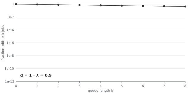
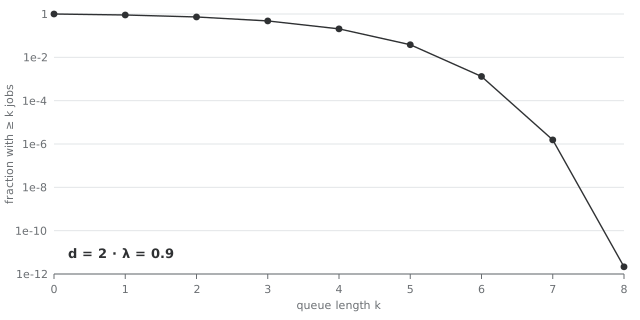
Figure 2. Classical baseline, not a project result. The mean-field fixed point of the textbook model at load $\lambda = 0.9$ , on the same log axis: drag the divider. With one sample per job the fraction of servers holding at least $k$ jobs falls only geometrically, $0.9^k$ , to 0.430 at $k = 8$ . With two it falls doubly exponentially, to about $1.5\times10^{-6}$ at $k = 7$ and $2.1\times10^{-12}$ at $k = 8$ . Closed form, no sampling. This is the typical picture, the mean-field limit; the rare event this project estimates lies outside it.

The Limit Against a Finite System

The fixed point is a statement about $n \to \infty$ . Figure 3 sets it against a seeded simulation of $n$ servers under the same textbook model. For $d = 1$ the closed form is exact at every $n$ in stationarity, so the simulation should land on it within its error bars; for $d \ge 2$ it is only the limit, and the widget shows how far a small system sits from it.

Figure 3. Classical baseline, not a project result or method. The mean-field closed form for a load $\lambda$ from 0.5 to 0.99 and $d \in \{1, 2, 3, 5\}$ , against a seeded event-driven simulation of $n \in \{10, 100, 1000\}$ servers under the textbook model above, assumed for illustration: Poisson arrivals at rate $\lambda n$ , unit-rate exponential service, and $d$ servers sampled uniformly with replacement. Points are time averages, $\pm 1$ s.e. across independent runs; the readout gives the seed. For $d = 1$ each server receives an independent Poisson( $\lambda$ ) stream, so each queue is an M/M/1 queue with load $\lambda$ and $\mathbb P(Q_i \ge k) = \lambda^k$ holds exactly at every $n$ in stationarity; each run starts from that law. For $d \ge 2$ the closed form is the $n \to \infty$ limit, and the gap at small $n$ is a stationary finite- $n$ correction. It is not the time-window rare event this project estimates.

Crude Monte Carlo and Importance Sampling

In symbols, crude Monte Carlo runs $M$ independent copies of the system and counts how often the event $A$ occurs. Its relative error is the standard deviation over the mean:

\hat p^{\,\mathrm{crude}}_M = \frac{1}{M}\sum_{j=1}^M \mathbf 1_A(\omega_j),\qquad \mathrm{RE} = \sqrt{\frac{1-p}{M p}} \;\Longrightarrow\; M = \frac{1-p}{p\,\mathrm{RE}^2}.

An event of probability $10^{-20}$ needs something like $10^{22}$ independent replications before the estimator has a usable relative error.

Reading "usable" as a 10% relative error, the formula gives $M \approx 10^{22}$ runs at $p = 10^{-20}$ .

Importance sampling draws the runs from a modified law $Q$ instead and reweights each one by the likelihood ratio, which keeps the estimate unbiased:

p = \mathbb{E}_P[\mathbf 1_A] = \mathbb{E}_Q\!\Big[\mathbf 1_A \tfrac{dP}{dQ}\Big],\qquad \hat p^{\,\mathrm{IS}}_M = \frac1M \sum_{j=1}^M \mathbf 1_A(X_j)\,\frac{dP}{dQ}(X_j),\quad X_j \sim Q.

Everything then depends on choosing $Q$ well.

The Mechanism, on a Target with a Known Answer

Figure 4 runs both estimators on the Gaussian tail $\mathbb P(Z > a)$ , $Z \sim \mathcal N(0,1)$ , whose exact value $\Phi(-a)$ , with $\Phi$ the standard normal distribution function, is known to machine precision. Shifting the mean to the threshold, $Q = \mathcal N(a,1)$ , makes the event common, and the weight is explicit:

\frac{dP}{dQ}(x) = \frac{e^{-x^2/2}}{e^{-(x-a)^2/2}} = e^{-a x + a^2/2},\qquad \hat p = \frac1M \sum_{j} \mathbf 1\{X_j > a\}\, e^{-a X_j + a^2/2},\quad X_j \sim \mathcal N(a,1).

Fig. 4. The mechanism, on a target with a known answer. Estimating P(Z > a) for Z ~ 𝒩(0,1) by crude Monte Carlo (hollow) and by importance sampling under the tilted law 𝒩(a, 1) with weight exp(−aX + a²/2) (filled), against the exact Φ(−a), dashed. Both carry ±1 s.e. Watch crude Monte Carlo degrade rather than fail cleanly: its markers drift off the curve, go bright as the relative error climbs, survive on a single chance hit two decades out of place with an error bar spanning the axis, and then stop appearing. The tilted estimator tracks the exact curve five decades further down. The readout reports where each method last held a relative standard error under 50%. The reference comes from an erf series and the Laplace continued fraction, agreeing with SciPy to 7×10⁻¹⁵.

Figure 4. Classical baseline: a textbook instance, chosen because its answer is exact. It stands in for the mechanism and is not a project result: it does not touch the project's estimator.

Why the tilt works here. Write $W = e^{-aX + a^2/2}$ for the weight. Then

\mathbb{E}_Q\big[W^2 \mathbf 1\{X>a\}\big] = e^{a^2}\,\Phi(-2a),\qquad \frac{\operatorname{Var}_Q}{p^2} = \frac{e^{a^2}\Phi(-2a)}{\Phi(-a)^2} - 1 \;\sim\; a\sqrt{\pi/2}\quad (a\to\infty).

The relative variance per sample grows only polynomially in $a$ . For crude Monte Carlo it is $(1-p)/p$ , which grows like $e^{a^2/2}$ up to polynomial factors.

Key step, with $\varphi$ the standard normal density: $e^{-ax}\varphi(x) = e^{a^2/2}\varphi(x+a)$ , so $\int_a^\infty e^{-ax+a^2/2}\varphi(x)\,dx = e^{a^2}\Phi(-2a)$ . Textbook, and specific to this Gaussian stand-in.

How Figure 4 Is Checked

Figure 4 is one of the site's live simulations that a verification script checks against an exact reference before it ships:

Item	Value
Target	$\mathbb P(Z > a) = \Phi(-a),\ Z \sim \mathcal N(0,1)$
Thresholds	$a = 1, 1.5, \dots, 7$ (13 values)
Importance-sampling check	4,000,000 samples per threshold; $\|z\| \le 4$ against the exact value is required at every threshold; measured maximum 2.04
Exact reference against SciPy	worst relative difference $7.2\times10^{-15}$ (a recorded snapshot)
Seeds	`gaussian-tail/2026` for the live figure, `verify/raretail` for the check

From the site's repository:

node scripts/verify-raretail.mjs   # the check behind Figure 4
npm run verify                      # all of the site's verification scripts

Large Deviations Supply the Tilt

The decay rate of the probability, and the most likely path along which the rare event happens, are described by a rate function built from the Cramér transform of the per-server net input. Knowing how the system gets to the rare state tells us how to tilt the dynamics so that it goes there routinely. Figure 5 shows where that sits among the ways to spend $M$ runs.

Figure 5. Three ways to spend $M$ runs; the dots switch panels. Crude Monte Carlo under $P$ returns zero occurrences and no information about the magnitude. Importance sampling tilts the law so the event becomes common and reweights each run by $dP/dQ$ ; large-deviation theory says which tilt, and the Gaussian case is Figure 4. A badly chosen tilt can give infinite variance while the output looks fine ("a few rare runs carry huge weights" is a sketch of the mechanism). At the other extreme, the Doob $h$ -transform gives every run the same weight $p$ and zero variance, but building it requires $h$ , which is the unknown probability itself, so in practice the optimal tilt has to be approximated.

The ingredients, in textbook form. For a per-server net input $Y$ , the log moment generating function and its Cramér transform are

\Lambda(\theta) = \log \mathbb{E}\, e^{\theta Y},\qquad \Lambda^*(y) = \sup_{\theta \in \mathbb R}\big\{\theta y - \Lambda(\theta)\big\}.

For the empirical measure, the generic shape of a large-deviation principle on path space is

\mathbb{P}\big(\mu^n \in \Gamma\big) \approx \exp\!\Big(-n \inf_{\psi \in \Gamma} I_T(\psi)\Big)

for a set $\Gamma$ of measure-valued paths, with a rate function $I_T$ on the horizon $T$ ; precisely, an upper bound for closed sets and a lower bound for open ones. The net input $Y$ for this model, its rate function and the tilt built from it are held back with the manuscript.

The textbook shape, not a result stated here for this model. It concerns events of the empirical measure $\mu^n$ , a macroscopic object.

The Optimal Tilt Is a Doob h-Transform

The optimal tilting is characterized by a Doob $h$ -transform of the underlying chain. For a continuous-time chain with rates $q(x,y)$ , a target set $B$ with hitting time $\tau_B$ , and a horizon $T$ , let $h(t,x) = \mathbb P(\tau_B \le T \mid X_t = x)$ . Then

q^h_t(x,y) = q(x,y)\,\frac{h(t,y)}{h(t,x)},\qquad \frac{dP}{dQ^h}\Big|_{\{\tau_B \le T\}} = h(0,x_0) = p\ \text{ on every path}\;\Longrightarrow\; \operatorname{Var}_{Q^h}(\hat p) = 0 .

Every path that reaches $B$ returns the same weight, so the estimator has zero variance. The catch is that $h$ is the unknown itself, which is why in practice it has to be approximated. How we build our tilt is held back pending submission.

Key step, time-homogeneous case ( $T = \infty$ ): $h$ is harmonic on the transient states, so the total exit rate is unchanged and the likelihood ratio telescopes to $h(x_0)/h(x_\tau) = h(x_0)$ .

What Efficient Means

A standard yardstick for a rare-event estimator is logarithmic efficiency: on the exponential scale, its second moment decays twice as fast as the probability itself,

\liminf_{n\to\infty} \frac{\log \mathbb{E}_Q\big[(\hat p_n)^2\big]}{\log p_n} \;\ge\; 2,

which is the best possible, since by Jensen's inequality the ratio is at most 2. Whether an estimator built this way is genuinely efficient, or only assumed to be, is one of the questions we ask.

Large-deviation tools reach past queueing: Sanov's theorem and the Donsker–Varadhan variational formula for relative entropy are the machinery behind PAC-Bayes generalization bounds. That is context for why the tools are worth knowing, not a claim about what this project does.

Exact Against Asymptotic

Methodologically, we commit to not taking any of that on faith. The estimators run on a reproducible Python simulation framework with deterministic seeding, and they are checked against crude Monte Carlo wherever crude Monte Carlo is reliable. For system sizes where it is still feasible, the probability can be computed exactly rather than estimated: uniformizing the killed chain reduces the question to linear algebra on the occupancy state space, which gives ground truth with no sampling error. With $B$ made absorbing, $G_B$ the resulting generator, a rate $\nu \ge \max_x |G_B(x,x)|$ and $\tilde P = I + G_B/\nu$ ,

\mathbb{P}_x(\tau_B \le T) = \sum_{m=0}^{\infty} e^{-\nu T}\frac{(\nu T)^m}{m!}\,\big(\tilde P^{\,m}\mathbf 1_B\big)(x).

Every term lies in $[0,1]$ , so truncating the Poisson sum leaves a Poisson tail as an explicit error bound. The remaining errors are truncation and rounding, never sampling. It is feasible only at small $n$ .

Figure 6. Exact, asymptotic and estimated answers to the same question, with the question each pair of them answers. Exact computation is feasible only at small $n$ ; at large $n$ only estimates remain, which is why the exact answer has to be on hand wherever it can be. The diagram carries no numbers: these comparisons are what the project commits to, and their results are held back.

Against that ground truth we can ask the questions that otherwise get waved through. Has the asymptotic rate actually taken hold at the system sizes anyone simulates? Is the estimator genuinely efficient, or only assumed to be? Do the approximations made in deriving the tilting cost anything that shows up in practice? Of the three, exact against asymptotic is the comparison I find most worth doing.

Current Status

The project is paused while Ruoyu Wu is on sabbatical. It has run since November 2024, as an Undergraduate Research Fellowship in the Department of Mathematics at Iowa State, with a Dean's High Impact Undergraduate Research Award (2026). Our manuscript, Large-Deviation-Guided Importance Sampling for Rare Events in the Mean-Field Join-the-Shortest-Queue Model, is on hold until the project resumes. The table below sets what this page shows against what is held back pending submission.

On this page	Held back pending submission
The setting and the problem, in the words of the public write-up	The precise rare event and the model's parameters
The textbook definitions this page uses: the importance-sampling identity, the Cramér transform, the $h$ -transform, uniformization, logarithmic efficiency	How the project's change of measure is constructed
Classical baselines with exact references (Figures 2 to 4)	Every result of the project
The site's check for Figure 4, which can be rerun from the site's repository	The code and the manuscript text

The code is in a private repository.

Langevin Sampling All research Learned PDE Solvers